Bayesian analysis (but not pure Bayes factor analysis) allows clear reporting of error probabilities

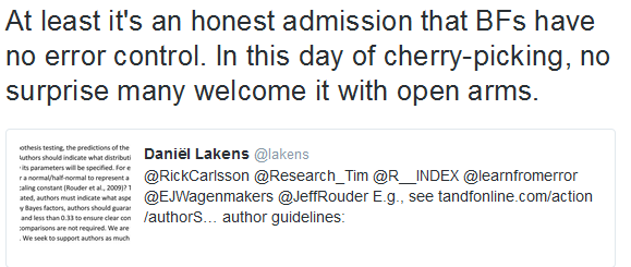
I noticed this exchange on Twitter last week. Daniel Lakens posted a screenshot from the reviewer guidelines of Comprehensive Results in Social Psychology. The guidelines promote Bayes factor analysis, and in particular accepting a hypothesis when the Bayes factor in favour of that hypothesis is greater than 3. 

Deborah Mayo responded criticising this approach for lacking error control:

I’ve noticed variations on this argument – that Bayes factor analyses lack error control - floating around a fair bit over the last while. Being a Bayesian myself (mostly), and being concerned about making errors in inference, I figured it might be useful to sort through my thoughts on this issue and post some relevant points.

Point 1: Frequentist significance tests involve decision rules that control error rates; Bayesians report the probability of error
Significance tests - or at least most types of them - involve a decision rule set up in such a way that it will control the rate of some type of error. Almost always, the decision rule will be set up to keep the probability of a Type 1 error (a false rejection of the null hypothesis) to 5%. The decision rule is typically intended to be a rigid and intrinsic part of the analysis: We reject the null hypothesis if p < .05, and do not reject it if not.

On the other hand, in a Bayesian analysis, we don't necessarily have to apply some firm decision rule. A Bayesian analysis is capable of providing a statement like "Given the priors specified and data observed, there is an 85% probability that this hypothesis is correct". (A statement which implies, in turn, a 15% chance of being in error if one was to decide in favour of the hypothesis). A researcher reporting a Bayesian conclusion like the one above could leave simply it at that; they could apply a decision rule (e.g., posterior probability > 90% is required to support a hypothesis), but they don't have to. Therefore, because a significance test is essentially a decision rule while Bayes theorem isn't, it is probably best to say that a frequentist analysis seeks to control error rates, while a Bayesian analysis will communicate the error probability (i.e., the probability that a particular conclusion would be incorrect). Both of these approaches seem to be reasonable alternatives to me. But what are we assuming when we report error probabilities in this Bayesian way?

Point 2: Frequentist and Bayesian approaches are both concerned with the probability of error, but they condition on different things

Frequentist hypothesis tests are typically aimed at controlling the rate of error, conditional on a particular hypothesis being true. As mentioned above, a statistical significance test for a parameter is almost always set up to such that conditional on the null hypothesis being true, we will erroneously reject it only 5% of the tim.

The situation in a Bayesian analysis is a bit different. A Bayesian test of a hypothesis produces a posterior probability for that hypothesis. We can subtract this posterior probability from 1 to get an error probability. But this error probability isn't the probability of error, conditional on a particular hypothesis being true; it's the probability that a particular conclusion is incorrect, conditional on the priors specified and data observed.

So we have two types of error probabilities: The probability of error conditional on a hypothesis, and the probability of error conditional on the prior and observed data. Both of these are perfectly reasonable things to care about. I don’t think it’s reasonable for anyone to dictate that researchers should care about only one of these.

For me personally, once I’ve finished collecting data, run an analysis, and reached a conclusion, I’m most interested in the probability that my conclusion is wrong (which is part of the reason why I’m keen on Bayesian analysis). But this doesn’t mean I’m completely disinterested in error rates conditional on particular hypotheses being true: This is something I might take into account when planning a study (e.g., in terms of sample size planning). I’m also broadly interested in how different types of Bayesian analyses perform in terms of error rates conditional on hypotheses. Which leads me to the next point...

Point 3: An analysis may focus on one type of error probability, but we can still study how it performs in terms the other.

A frequentist significance test will typically be set up specifically to control the rate of falsely rejecting the null, conditional on the null hypothesis being true, to 5% (or some other alpha level). But this doesn’t mean we can’t work out the probability that a specific conclusion is incorrect, conditional on the data observed (i.e., the Bayesian type of error probability). Ioannidis’ paper claiming that most published research findings are false deals with exactly this problem (albeit based on some shaky assumptions): He calculated the probability that an effect actually exists, conditional on a significant test statistic, for a range of priors and power scenarios. There is admittedly a bit of a conceptual problem here with trying to draw Bayesian conclusions from a frequentist test, but the mathematics are fairly straightforward.

Similarly, while a Bayesian analysis is set up to tell us the probability that a particular conclusion is in error, given the priors set and data observed, there’s no reason why we can’t work out the rate at which a Bayesian analysis with a particular decision rule will result in errors, conditional on a particular hypothesis being true. This previous blog of mine is concerned with this kind of problem, as are these better ones by Daniel Lakens, Alex Etz and Tim van der Zee.

The upshot is that while a particular type of analysis (frequentist or Bayesian) may be tailored toward focusing on a particular type of error probability, we can still use a bit of mathematics or simulation to work out how it performs in terms of the other type. So choosing to focus on controlling one type of error probability hardly implies that a researcher is disregarding the other type of error probability entirely.

Point 4: The Bayesian error probability depends on the prior

A word of caution about Bayesian error probabilities: Given its dependence on a prior, the type of inference and error rate I get with a Bayesian analysis is useful primarily provided I can set a prior that’s relevant to my readership. If I set a prior where most of the readers of my study can say “yes, that seems a reasonable description of what we knew in advance”, and I draw a conclusion, then the posterior probability distribution tells them something useful about the probability of my conclusion being in error. But if they think my prior is utterly unreasonable, then I haven’t given the reader direct and useful information about the chance that my conclusion is wrong.

Point 5: Back to that editorial recommendation of support H₁ if BF₁₀>3

Finally I want to reflect on how error probabilities are dealt with in a very specific type of analysis, which is a Bayes factor analysis using a default prior for the H1 model, and a decision rule based solely on the Bayes factor rather than a posterior probability distribution. This is more or less the type of analysis recommended by the “Comprehensive Results in Social Psychology” editorial policy that started off this whole discussion.

Now in this case, the analysis is not set up to control the rate of error, conditional on a particular hypothesis being true, to a specific value (as in a frequentist analysis). However, because it doesn’t involve a commitment to a particular prior probability that the null hypothesis is correct, it also doesn’t directly tell us the probability that a particular conclusion is false, conditional on the data (the Bayesian type of error probability).

This latter problem is reasonably easily remedied: The author can specify prior probabilities for the null and alternate, and easily calculate the posterior probability that each hypothesis is correct (provided these prior probabilities sum to 1):

Posterior odds = P(H1)/P(H0) * BF_H1

P(H1|Data) = Posterior odds/(1+posterior odds)

For example, say we're doing a t-test and take an uber-default assumption of P(H0) = P(H1) = 0.5, with a Cauchy (0, 0.707) on standardised effect size under H1 (the JASP default, last time I checked). We then observe a BF₁₀ of 3. This implies a posterior probability of 3/4 = 75% in favour of H1. In other words, if you observed such a Bayes factor and concluded in favour of the alternate, there'd be a 25% chance you'd be in error (conditional on the data and prior specification). 

That said, this error probability is only informative to the extent that the priors are reasonable. The prior used here takes a spike-and-slab prior form which implies that there's a 50% chance the effect size is exactly zero, yet a substantial chance that it's extremely large in size (e.g., a 15% prior probability that the absolute true effect size is greater than 3). A reader may well see this prior probability distribution as an unreasonable description of what is known about a given parameter in a given research setting.

So I think it is crucial that authors using Bayes factor analyses actually report posterior probabilities for some reasonable and carefully selected priors on H1 and H0 (or even a range of priors). If this isn’t done, the reader isn’t provided with direct information about either type of error probability. Of course, a savvy reader could assume some priors and work both types of error probability out. But I think we have an obligation to not leave that entire process to the reader. We should at least give clear information about one of the types of error rates applicable to our study, if not both. So I disagree with the reviewer guidelines that provoked this post: We shouldn't make statistical inferences from Bayes factors alone. (If you use Bayes factors, make the inference based on the posterior probability you calculate using the Bayes factor).

Secondly, the priors we set on H0 and H1 (and the prior on effect size under H1) in a Bayes factor analysis should be selected carefully such that they're a plausible description of what was known ahead of the study. Otherwise, we'll get a posterior probability distribution and some information about the probability of error, but this probability of error will be conditional on assumptions that aren't relevant to the research question nor to the reader.

Lots of problems with the Reliable Change Index

In a previous post, I talked about the Reliable Change Index (RCI: Jacobson & Truax, 1991), and a rather unusual misconception about its implications.

Today, as I promised in that earlier post, I want to talk about the RCI a bit more broadly, and discuss some problems with its use. (TL;DR: The RCI doesn't test the hypothesis we're interested in, and has extremely poor statistical power for testing the hypothesis that it does).

Introduction to the RCI

For those who haven't heard of it, the RCI is something that's popular amongst clinical psychologists conducting single case experimental designs. Basically the idea is:

• We obtain a pre score on the measure of interest for our lone participant, administer an intervention, then obtain a post score, and calculate the observed difference between the two. (I.e., how much did the participant improve?)
• Using reliability and variability estimates from a psychometric validation study of the measure (or whatever is available), we calculate the standard error of measurement of a set of scores: SEM = SD*sqrt(1 - reliability)
• Using the SEM, we calculate the standard error of measurement of the difference between pre and post scores: Sdiff = sqrt(2*SEM^2)
• We compare the observed improvement in the participant's score to the critical ratio 1.96*Sdiff; if it is greater than this critical ratio, the improvement is "reliable"/statistically significant.

Now collecting large samples of data for trials of psychotherapy interventions is a pretty expensive and painful process, so single case experimental designs are still reasonably popular in clinical psych (well, at least here in New Zealand they are). And to be able to do a single case experimental design and yet still run a proper objective inferential statistic has its appeal - it feels much more objective than all that business of just qualitatively interpreting plots of single case data, doesn't it?

What the RCI does and doesn't test

However, while the RCI is indeed an inferential statistic, I'm not sure that it allows you to make an inference about anything you really care about.

Consider, first of all, the null hypothesis that the RCI is testing. The null hypothesis is that the participant's true score at time 1 was the same as her true score at time 2. What is a true score on a measure? Well, a true score is a concept from classical test theory. Specifically, a true score is the average score the participant would get if we could administer the measure to the participant an infinite number of times, with each administration being independent of the others (i.e., we'd have to wipe their memories after each administration), and without their actual level of the measured attribute changing (so imagine a counterfactual world where we could keep administering the measure repeatedly at exactly the same point in time). Importantly, the true score is not the participant's actual level of the attribute we're trying to measure.

So the true score is an abstract and rather strange concept; I'm not sure we really care about whether a participant's true score has changed after the intervention. Rather, the key question is: Did the intervention cause a change in the person's actual level of the attribute of interest?

Now the RCI does actually relate to that causal question, in the sense that it helps to rule out one specific alternative explanation for an observed difference in scores: It helps us rule out the possibility that a difference we've seen is purely due to random measurement error.

But the problem is that it doesn't help us rule out any much more pressing alternative explanations (other than an actual causal effect of the intervention). These alternative explanations include:

• Maturation: The change in scores could be due to some natural time-related process (e.g., aging)
• History: The change in scores could be due to some external event not caused by the intervention
• Regression to the mean: The change in scores could be due to the selection of a participant with an extreme observed level of the variable of interest, who in probability would receive a less extreme score on re-testing (regardless of intervention)
• Testing: The sheer act of taking the pre-test measurement could have the participant
• Instrumentation: There could have been a change in the measurement method in the intervention period (related to the idea of systematic measurement error, which the RCI does not address)

All of these threats to internal validity are just as pressing as the threat of random measurement error, but the RCI doesn't address any of them. In fact, the RCI does not even address the issue of whether or not there is some kind of enduring change to explain at all. If the actual attribute of interest (e.g., depression, anxiety) fluctuates from day to day (as distinct from fluctuation due to measurement error), there might be a difference in true scores between two measurement occasions, but without any enduring change whatsoever in the person's typical level of the attribute of interest.

Power problems

Unfortunately, even if we accept that the RCI doesn't really tell us what we are most interested in knowing, and we're willing to accept making inferences only about differences in true scores rather than causal effects, there is still a major lurking problem. That problem is that in realistic conditions, the RCI has absolutely abysmal statistical power. A plot showing statistical power relative to effect size for measures of various levels of reliability is shown in the figure below.

As you can see, the picture is very worrying: You can achieve 80% power only if the effect size is large and the reliability of your measure stupendous (e.g., effect size d of around 0.8 and reliability of 0.95). In more realistic circumstances - say a medium effect size of d = 0.5 and reliability of 0.8 - your power is well under 30%. And with measures of lower reliability and smaller effects, the statistical power of the test is barely higher than the Type 1 error rate. In these circumstances, even if by some magical coincidence we do come across a significant result, we shouldn't place any trust in it: the lower the power, the lower the probability that a significant finding reflects a true effect (see Ioannidis, 2005).

Why is the power of the RCI so low? Well there's no getting away from the fact that in a single case study, N = 1. By deliberately focusing only on ruling out measurement error variation (rather than all extraneous variation) we increase the power of the test a little, but the reality is that two measurements from a single person simply can't allow us to make precise inferences.

Assumptions

And we can go further down the rabbit hole still: There are three more specific distributional assumptions that are problematic in regard to the RCI:

1. The RCI may be biased if it is based on an estimate of reliability whose distributional assumptions were not met (which is likely to be the case if it is based on a Cronbach's alpha estimate)
2. The RCI is based on the assumption that the measurement error variance is constant across people, and specifically that the quantity of measurement error is the same for your participant as it is in the sample you got your reliability estimate from. If, as could very well be the case, measurement error is higher or lower for your participant than that estimate, then the RCI will give biased inferences.
3. The RCI is based on the assumption that the measurement error for your participant is normally distributed over testing occasions. If this (untestable) assumption does not hold, the fact that N = 1 means that there is no protection to be gained from the central limit theorem. Consequently small departures from normality could distort Type 1 error rates.

So what to do? 

While I totally respect the intentions of those trying to use the RCI to add rigour to single case experimental designs, I'm not sure that the RCI is worth reporting. It doesn't really address the real question of interest in a single case experimental design, and its poor power means that it's likely to produce untrustworthy inferences.

But what to report instead? If you're wedded to a single case design, I think a couple of strategies that might help are:

• Collect lots of data points. If we can see how variable an individual participant's scores are within the baseline and intervention periods, this gives a much more direct (albeit subjective) impression of whether random fluctuation in scores could account for an observed difference between baseline and treatment. And with a very large number of data points collected at regular intervals you may even be able to use methods designed for time series data (e.g., change point regression) to detect a change in behaviour at the time of the intervention.
• If you can, use a withdrawal design (e.g., ABAB). Hell, if you can go back and forth between treatment and baseline a bunch of times at random, you could even run a perfectly conventional significance test to compare the two conditions. Unfortunately I don't think this is a feasible option for the types of intervention most psychologists are interested in nowadays though (you can't "withdraw" teaching the participant how to practice mindfulness, say).

But at the end of the day, I think there's no getting around the fact that making quantitative claims on the basis of data from a single participant is a pretty risky process. If you're trialling an intervention with one of the H.M.s of the world - someone whose condition is so rare you just can't possibly get a decently sized sample even in principle - then stick with a single case design and make do. But if the reality is that you just want to trial a psychotherapy with people who have a reasonably common condition - and you're using a single case design only because running a large sample RCT is beyond your current means - then I think it's worth re-thinking things more completely and considering whether another research topic might be more deserving of your attention.

Appendix: R code for plot

For a Type 1 error rate of 5%, accept H1 if BF10 > 1 (wait, what?)

So I was looking at Daniel Lakens' fascinating recent blog post The Dance of the Bayes Factors, where he shows how Bayes factors are subject to a pretty substantial degree of sampling variability. When used as a basis for a decision about whether a null hypothesis is true or false, they can also (of course) result in errors. For example, Daniel shows that for a two-sample comparison of means, with n = 75 in each group and a true effect size of Cohen's δ = .3, quite high rates of Type 2 errors can result. In particular, Daniel notes that we will:

• Falsely support the null 25% of the time if we set a cutoff of BF10 < 1/3 for supporting the null
• Falsely support the null 12.5% of the time if we set a stricter cutoff of BF10 < 1/10 for supporting the null

I wondered: What kind of Type 2 error rate would result if we set our evidence cut-offs so as to ensure a Type 1 error rate of 5%? To figure this out, I simulated some data where the null is true, and where we again have n of 75 in each group, and see what cut-off would preserve this Type 1 error rate:

require(BayesFactor) 

set.seed(123)
get.BF = function(cohensd, n){
  x<-rnorm(n = n, mean = 0, sd = 1) #produce N simulated participants
  y<-rnorm(n = n, mean = cohensd, sd = 1) #produce N simulated participants
  z<-t.test(x,y) #perform the t-test
  BF10<-exp(ttest.tstat(z$statistic,n,n,rscale=sqrt(2)/2)$bf)
  BF10
}
simsH0 = replicate(10000, get.BF(cohensd = 0, n = 75))
quantile(simsH0, probs = 0.95)

##       95% 
## 0.9974437

Wait… what? It turns out that even if we accept any Bayes factor greater than 1 as a basis to support H1, we will only reject H0 falsely 5% of the time! That seems bizarre - a Bayes factor of 1, after all, means that the data is just as consistent with H0 as it is with H1! (Note: The cut-off for a 5% error rate differs according to the H1 prior specified and the sample size - don't take the title of this post too literally!)

How about if we used stricter cut-offs of BF10 > 3 (“positive” evidence according to Kass and Raftery, 1995), or > 20 (“strong” evidence)?

sum(simsH0 > 3)/length(simsH0)

## [1] 0.0114

sum(simsH0 > 20)/length(simsH0)

## [1] 0.0015

It turns out that if we use the BF10 > 3 criterion (which still seems very liberal), our Type 1 error rate is only about 1%. And it we use a rule of BF10 > 20 as a cut-off for supporting H1, our Type 1 error rate becomes absolutely miniscule - about 0.15%.

Weird. But let's follow this exercise to its conclusion… what Type 2 error rate results if we the BF10 > 1 rule to support H1? Well, presuming Daniel's original effect size of δ = 0.3:

simsH1 = replicate(10000, get.BF(cohensd = 0.3, n = 75))
sum(simsH1 > 1)/length(simsH1) #We support H1 46% of the time

## [1] 0.4621

power.t.test (75, 0.3) #Which is virtually identical to the power of a frequentist t-test

## 
##      Two-sample t test power calculation 
## 
##               n = 75
##           delta = 0.3
##              sd = 1
##       sig.level = 0.05
##           power = 0.4463964
##     alternative = two.sided
## 
## NOTE: n is number in *each* group

So, on one level, we have a reassuring result: It is possible to set a Bayes factor cut-off for “decisiveness” that gives us basically the same Type 1 and Type 2 error rates as a conventional significance test. Which makes sense: The Bayes factor is just a monotonic transformation of the p value, after all.

But on the other hand… a lot of this doesn't make a lot of intuitive sense. How can we maintain a low Type 1 error rate with such a liberal cut-off for supporting H1? And why does the same incredibly liberal cut-off not result in particularly good power for supporting H1 when the true effect size is small but definitely not zero?

The answer to this lies in thinking about the models we're actually comparing here. We might think of this test as comparing an hypothesis of an exactly zero effect (H0) to one of a non-zero effect (H1), but that isn't actually what we're doing. The H1 model being tested is that the true effect size δ is randomly drawn from a Cauchy distribution with location = 0 and scale = 0.707.

Now when the true effect size δ is zero, the majority of sample effect sizes we see are indeed near zero. And the null (H0) model tends to fit the resulting sample estimates quite well, as it should (since it's the true model). On the other hand, the H1 model of Cauchy (0, 0.707) is quite spread out: It implies a 50% chance of an effect size |δ| > 0.707. Correspondingly it suggests that sample effect sizes very near zero are quite improbable. So when H0 is true, the H1 model tends not to fit the data well, and we will accidentally support it only very rarely.

But what's the story when the true effect size is δ = 0.3? Why is the Bayes factor test still so shy to support the H1 model, even if the null hypothesis is actually false, and even if we take the slightest sliver of evidence (BF10 > 1) as enough to say H1 is true?

Well, first of all, in this situation neither the H0 model nor the H1 model is true. The H1 model suggests that the true effect size is randomly drawn from a Cauchy distribution, and places zero prior probability on the true effect size taking any specific point value. But here the true effect size is a fixed, small, value. So both models are technically false, but either could sometimes fit the resulting data quite well. And, as it happens, because the H1 model of Cauchy (0, 0.707) suggests that a small true effect size isn't very probable, it tends not to fit very well to data simulated according to a fixed, small, effect size. On the other hand, the null model often fits reasonably well with such data. Hence in this situation we tend to be much more likely to support H0 than H1, even though H0 is false.

In one sense, the result I come up with above is just a statistical curiousity, and one that probably won't be very surprising to people very familiar with Bayes factors. But I think there are some simple philosophy-of-science considerations to keep in mind here that might be of interest to some.

Basically, when we use a Bayes factor test of a null hypothesis test, the H1 model we specify is a falsifiable (but literally false) model that we use as a stand-in for the possibly-true (but unfalsifiable) substantive hypothesis: That the true effect size simply isn't zero. That isn't a fault of the test: No statistical test can make up for the fact that psychological hypotheses are often too vaguely specified to be directly tested without being reformulated. But we need to be wary of over-interpreted a Bayes factor result that supports the null hypothesis: Such a result implies that H0 fits the data better than the specific H1 model we've specified… but it doesn't necessarily mean the null hypothesis is true.

No, a breach of normality probably won't cause a 17% Type 1 error rate

Over the weekend I came across this article on the PsychMAP Facebook group

Cain, M. K., Zhang, Z., & Yuan, K.-H. (2016). Univariate and multivariate skewness and kurtosis for measuring nonnormality: Prevalence, influence and estimation. Behavior Research Methods. https://doi.org/10.3758/s13428-016-0814-1

From the abstract:
"this study examined 1,567 univariate distriubtions and 254 multivariate distributions collected from authors of articles published in Psychological Science and the American Education Research Journal. We found that 74 % of univariate distributions and 68 % multivariate distributions deviated from normal distributions. In a simulation study using typical values of skewness and kurtosis that we collected, we found that the resulting type I error rates were 17 % in a t-test and 30 % in a factor analysis.  Hence, we argue that it is time to routinely report skewness and kurtosis..."


Hang on... a 17% Type I error rate purely due to non-normality? This seemed implausibly high to me. In an OLS model such as a t-test (or ANOVA, or ANCOVA, or regression, or whatever), the assumption of normally distributed error terms really isn't very important. For example, it isn't required for the estimates to be unbiased or consistent or efficient. It is required for the sampling distribution of test statistics such as the t statistic to follow their intended distributions, and thus for significance tests and confidence intervals to be trustworthy... but even then, as the sample size grows larger, as per the CLT these sampling distributions will converge toward normality anyway, virtually regardless of the original error distribution. So the idea of non-normal "data" screwing up the Type 1 error rate to this degree was hard to swallow.

So I looked closer, and found a few things that bugged me about this article. Firstly, in an article attempting to give methodological advice, it really bugs me that the authors misstate the assumptions of OLS procedures. They say:

" we conducted simulations on the one-sample t-test, simple regression, one-way ANOVA, and confirmatory factor analysis (CFA).... Note that for all of these models, the interest is in the normality of the dependent variable(s)."

This isn't really true. We do not assume that the marginal distribution of the dependent variable is normal in t-tests, regression, or ANOVA. Rather we assume that the errors are normal. This misconception is something I've grumbled about before. But we can set this aside for the moment given that the simulation from the article that I'll focus on pertains to the one-sample t-test, where the error distribution and the marginal distribution of the data coincide.

So let's move on to looking at the simulations of the effects of non-normality on Type I error rates for the one-sample t-test (Table 4 in the article). This is where the headline figure of a "17%" Type 1 error rate comes from, albeit that the authors seem to be mis-rounding 17.7%. Basically what the authors did here is:

• Estimate percentiles of skewness and (excess) kurtosis from the data they collected from authors of published psychology studies
• Use the PearsonDS package to repeatedly simulate data from the Pearson family of distributions under different conditions of skewness and sample size
• Run one-sample t-tests on this data.

There are a number of conditions they looked at, but the 17.7% figure comes about when N = 18 and skewness = 6.32 (this is the 99th percentile for skewness in the datasets they observed).

However,  they also note that "Because kurtosis has little influence on the t-test, it was kept at the 99th percentile, 95.75, throughout all conditions." I'm unsure where they get this claim from: to the extent that non-normality might cause problems with Type 1 error, both skewness and kurtosis could do so. On the face of it, this is a strange decision: It means that all the results for the one-sample t-test simulation are based on an extremely high and unusual level of kurtosis, a fact that is not emphasised in the article.

As it happens, one of the real reasons why they chose this level of kurtosis is presumably that the simulation simply just wouldn't run if they tried to combine a more moderate degree of kurtosis with a high level of skewness like 6.32. The minimum possible kurtosis for any probability distribution is skewness^2 + 1.

That technical note aside, the net effect is that the headline figure of a Type I error rate of 17% is based on a tiny sample size (18) and an extremely unusual degree of non-normality: An extremely high degree of skewness (6.32, the 99th percentile for skewness across their observed datasets), and an extremely high degree of excess kurtosis (95.75, again the 99th percentile). To give you an idea of what this distribution looks like, check the histogram below (10,000 data points drawn from this distribution). It's a little hard to imagine even a very poor researcher not noticing that their is something amiss if this was the distribution of their raw data!

In fact, it's worth noting that the authors "contacted 339 researchers with publications that appeared in Psychological Science from January 2013 to June 2014 and 164 more researchers with publications that appeared in the American Education Research Journal from January 2010 to June 2014", but we have no idea how many of these authors applied analyses that actually assumed normality. No doubt, some of the extreme levels of skewness and kurtosis arose in cases such as reaction time measurements or count data, where even without checking diagnostics the original authors might have been well aware that a normality assumption was inappropriate.

So what about more plausible degrees of non-normality? If anything, a close read of the article shows how even quite dramatic non-normality causes few problems: For example, take the case of N = 18, skewness of 2.77 and excess kurtosis of 95.75 (a small sample size with still quite extreme non-normality, as visualised in the q-q plot below - albeit not as extreme as the case discussed previously). The authors find that the Type 1 error rate (with alpha of 0.05) in this scenario is... 6.4%. That's hardly something to get too stressed out about!



Ok, so non-normality only really causes Type I problems in extremely severe situations: E.g., pathologically high levels of skewness and kurtosis combined with small sample sizes. But why am I picking on the authors? There is still at least some small danger here of inflated Type 1 error - isn't it good to be conservative and check for these problems?

Well, I have two main worries with this perspective.

Firstly, it's my perception that psychologists worry far too much about normality, and ignore the other assumptions of common OLS procedures. E.g., in descending order of importance:

• Conditional mean of errors for any combination of predictors are assumed to be zero (breached if correlated measurement error present, or any measurement at all in the Xs, or randomisation not conducted, or unmodelled non-linear relationships present between Xs and Y)
• Error terms are assumed to be independent
• Error terms are assumed to have the same variance, regardless of the levels of the predictors.

Now breaches of some of these assumptions (especially the first one) are much more serious, because they can result in estimates that aren't unbiased and consistent and efficient; consequently Type I error rates can of course be substantially inflated (or deflated). As methodologists, we need to bang on about normality less, and the other assumptions more. As Andrew Gelman has said, normality is a minor concern in comparison to some of the other assumptions (note that his phrasing of the OLS/regression assumptions is a little different to how I've written them above, though the ideas are similar).

Secondly, I worry that by encouraging researchers to check for non-normality (and then potentially change their analysis method if problems are found), we introduce extra researcher degrees of freedom into the analysis process. Deciding whether error non-normality is present is a subjective and challenging task, and there are many potential solutions to non-normality researchers can try. It thus strikes me that the potential for selective reporting (and even p-hacking) involved in encouraging researchers to check for non-normality and then attempt various remedies is actually a much greater threat to validity than any direct effect of non-normality.

In conclusion...Non-normality can cause problems, but only in very unusual situations. If you're running a t-test or regression, chances are that there are more important things for you to be worrying about.

What if the mean difference less than the standard error of measurement?

[Warning: Very Basic Stuff contained within]

Last weekend I was at a conference where there was an interesting tutorial-style talk on the Reliable Change Index (RCI). The RCI is generally used to try and determine if a single person has displayed 'real' change over the course of some intervention. (In other words, could an observed change in score plausibly have occurred purely due to random measurement error?)

I have some conceptual problems with the RCI in terms of whether it really tells us anything we really want to know (which I'll save for another day), but it was an interesting and well-delivered presentation. That said, I want to pick on an idea that was mentioned in the talk, and that I've heard others repeat recently.

The idea relates to extending the RCI outside of single cases. Particularly, the speaker suggested that when looking at a group study, that if a mean difference is less than the standard error of measurement, that this suggests that the apparent effect might be spurious (i.e., purely the result of measurement error) - even if the mean difference is statistically significant. His reasoning for this was that a statistical significance test focuses on sampling error, not measurement error.

Now, for a single case, a change in score that is less than the standard error of measurement is indeed one that would be quite consistent with a null hypothesis that the true score of the participant has not actually changed. (This isn't to say that this null is true, just that the observation isn't overtly unconsistent with the null). The RCI framework formalises this idea further by:

1. Using the SEM to calculate the standard error of the difference, Sdiff = sqrt(2*SEM^2). Since both the pre score and the post score are subject to errors of measurement, the standard error of the difference is a little more than the SEM.
2. Using 1.96*Sdiff as the cut-off for reliable change, drawing on the usual goal of a 5% Type 1 error rate.

All good so far. However, if we are comparing two sample means, the picture changes. At each time point we now have multiple observations (for different people), each with a different quantity of measurement error. The mean of the measurement error across people will itself have a variance that is less than the variance of the measurement error variable itself. This should be intuitively obvious: The variance of the mean of a sample of observations is always less than the variance of the underlying variable itself (well, provided the sample has N > 1 and the observations aren't perfectly correlated.)

In fact, when the sample is reasonably large, the standard error of the mean of the measurement error for the sample will be drastically less than the standard error of measurement itself. So an observation that a mean difference is less than the standard error of measurement is not necessarily consistent with the null hypothesis of no true change occurring.

So do we need to calculate the standard error of measurement for a particular sample, and use that along with a significance test (or Bayesian test) when assessing mean differences?

No.

Standard inferential tests do not only deal with sampling error. Any test you're likely to use to look at a mean difference will include an error term (often, but not necessarily, assumed to be normal and i.i.d. with mean zero). This error term bundles up any source of purely unsystematic random variability in the dependent variable - including both sampling error and unsystematic measurement error. So your standard inferential test already deals with unsystematic measurement error. Looking at the standard error of measurement in a group analysis tells you nothing extra about the likelihood that a true effect exists.

My talk at the M3 conference on Bayes factor null hypothesis tests

Recently I visited the USA for the first time. In between consuming vast quantities of pizza, Del Taco, and Blue Moon, I presented at the Modern Modeling Methods (M3) conference in Connecticut. (Slides included below).

The M3 conference was jam-packed full of presentations about technical issues relating to quite complex statistical models (sample presentation title: "Asymptotic efficiency of the pseudo-maximum likelihood estimator in multi-group factor models with pooled data"). The questions were serious, the matrix algebra was plentiful, and the word "SPSS" was never uttered.

My presentation was a little different: I wanted to talk about the default statistical methods used by everyday common-or-garden researchers: The ones who like t-tests, do their analyses by point-and-click, and think a posterior is something from a Nicky Minaj song (but may know lots and lots about things other than statistics!). I believe that the practices of everyday researchers are important to look at: If we want to fix the replication crisis, we need most researchers to be doing their research and analysis better - not just the ones who pass their time by discussing floating-point computation on Twitter.

And in terms of problems with the data analyses used by everyday researchers, the big issue that jumps out at me is the (mis)use of null hypothesis significance tests (NHST). Positions obviously vary on whether NHST should be used at all, but I think there's reasonable agreement amongst methodology geeks that the form of Fisher/Neyman-Pearson hybrid NHST that dominates current practice is really problematic. To me, a couple of the biggest problems are that:

1. Hybrid NHST (and frequentist analysis in general) doesn't directly tell us how certain we can be that a particular hypothesis is true. It tells us P(Data | Hypothesis), but we'd generally rather like to know P(Hypothesis | Data).
2. Hybrid NHST in specific has a problem with asymmetry of result: p < .05 is interpreted as meaning the null can be rejected, the alternate hypothesis is supported, publication results, and rejoicing is heard throughout the land. But p > .05 is often read as indicating only uncertainty: We can't say the null is true, only that there is insufficient evidence to reject it*. This may be a contributor to publication bias and the replication bias: Part of the preference against publishing null results may be that they are often interpreted as not actually communicating anything other than uncertainty.

But what do we replace hybrid NHST with? Abandoning inferential statistics entirely is obviously foolish. There are several options (Deborah Mayo's error statistics approach, Bayesian estimation, etc.) But an approach that's gaining especial traction in psychology at the moment is that of using Bayes factor tests: Particularly, using Bayes factors to compare the evidence for a point null vs. a vague alternate hypothesis (although obviously this isn't the only way in which Bayes factors can be used).

My talk was a gentle critique of this approach of Bayes Factor null hypothesis testing. And I do mean gentle - as I mention in slide 9 of the talk, I think Bayes factor tests of null hypotheses have some great advantages over conventional NHST. I mention several of these in my slides below, but perhaps the biggest advantage is that, unlike hybrid NHST, they compare two hypotheses in such a way that either hypothesis might end up supported (unlike NHST, where only the alternate can possibly "win"!) So I wouldn't want to stomp on the flower of Bayes factor testing. And certainly my talk critiques only a particular implementation of Bayes factors: To test a point null vs. a non-directional diffuse alternate. Much of the fantastic development of methods and software by guys like Rouder, Morey and Wagenmakers can be applied more broadly than just to Bayes factor tests of point null hypotheses.

But I do think that Bayes factor tests of point null hypotheses do have some problems that mean they may not be a suitable default approach to statistical analysis in psychology. (And currently this does seem to be the default way in which Bayes factors are applied).

To begin with, a Bayes factor is a statement only about the (ratio of) the likelihood of the data under the null and alternate hypotheses. It isn't a statement about posterior odds or posterior probabilities. For a Bayesian analysis, that seems to be a little unsatisfying to me. Researchers presumably want to know how certain they can be that their hypotheses are correct; that is, they want to know about posterior probabilities (even if they don't use those words). In fact, researchers often try to interpret p values in a Bayesian way - as a statement about the probability that the null is true.

And I suspect that a similar thing will happen if Bayes factor null hypothesis tests become commonplace: People will (at least implicitly) interpret them as statements about the posterior odds that the alternate hypothesis is correct. In fact, I think that kind of interpretation is almost supported by the availability of qualitative interpretation guidelines for Bayes factors: The notion that Bayes factors can be directly interpreted themselves - rather than converted first to posterior odds - seems to me to reinforce the idea that they're the endpoint of an analysis: that the Bayes factor directly tells us about how certain we can be that a particular hypothesis is correct. I know that Jeff Rouder has explicitly argued against this interpretation - instead saying that researchers should report Bayes factors and let researchers select and update their own priors (perhaps aided by suggestions from the researchers), and in an ideal world, that's exactly how things would work, but I don't think that this is realistic for everyday readers and researchers with limited statistical expertise.

So everyday researchers will naturally want a statement about the posterior (about how certain they can be that an hypothesis is correct) if doing a Bayes factor analysis. And I think it's likely that they will in fact interpret the Bayes factor as providing this information. But in what circumstance can a Bayes factor be interpreted as the posterior odds that the alternate hypothesis is correct? Well this is fairly obvious: The Bayes factor is the posterior odds that the alternate hypothesis is correct if we placed a prior probability of 0.5 on the null being true, and 0.5 on the alternate being true.

The thing is... that's a really weird prior. It's a prior that takes a "tower and hill" shape (see slides 13 and 14), and suggests that one particular value of the effect size (δ = 0) is vastly infinitely** more likely than any other value. It is absolutely and definitely a very informative prior, and yet also one that seems unlikely to represent our actual state of prior knowledge about any given parameter.

So this is a problematic prior - and when researchers use the Bayes factor as the endpoint of a statistical analysis without explicitly drawing on prior information, I would argue that this prior implicitly underlies the resulting conclusions. For this reason I don't think that a Bayes factor test of a point null hypothesis vs. a non-directional alternate, with the Bayes factor serving as the major statistical endpoint of the analysis, is an ideal default approach in psychology.

Ok... but what would be a better default approach? The relatively slight modification I suggested in the talk was to take into account the fact that most (not all) hypotheses tested in psychology are directional. Therefore, instead of focusing on the "strawman" of a point null hypothesis, we could focus on testing whether a particular effect is positive or negative.

This is most obviously achieved by using MCMC Bayesian estimation of a parameter and then tallying up the proportion of draws from the posterior that are greater than zero (i.e., the posterior probability that the effect is positive). However, it could also be achieved by using Bayes factors, by comparing an hypothesis that the effect is positive to an hypothesis that it is negative (with a half-Cauchy prior for each, say). So the statistical methods and programs (e.g., JASP) developed by supporters of Bayes factor testing could readily be adapted to this slightly altered goal. Either way, this would allow us to dispense with our inordinate focus on the point null, and directly test the hypothesis that's likely to be of most interest: that there is an effect in a specific direction.

However, in performing directional tests we need to take into account the fact that most effects in psychology are small: If we were to use uninformative priors, this would lead to excess confidence in our statements about the directionality of effects. That is, the posterior probability that the true effect is in the same direction as that found in the sample will be closer to 1 with an uninformative prior than it would be if we took into account the fact that most effects are small. I don't think it's feasible to expect everyday researchers to select their own informative priors, but methodologists could suggest default informative priors for psychology: Given that we know only that a particular parameter describes a psychological effect, which values of the parameter are most likely?

To achieve this, I suggest that we could find default prior variances for common analyses in psychology empirically. As a very rough idea of how this could work, I point out that Richard et al.’s (2003) meta-meta-analysis of 25,000 social psychological studies found a mean absolute effect of r = .23, which equates to a Cohen's d value of 0.43. We might use this information to set a default prior for a two-sample means comparison, for example, of Cauchy (0, 0.43), implying a 50% chance that the true standardised effect δ is somewhere between -0.43 and +0.43. (Note: There could be better choices of meta-meta-analysis to use that aren't restricted to social psych, and we would want to correct for publication bias, but this serves as a rough illustration of how we could set a default prior empirically). Use of this prior would allow us to make statements about the posterior probability that an effect is in a particular direction, without the statement being made overconfident due to use of an uninformative prior.

So that was my idea, and here are the slides from my presentation.

But. I'm definitely not perfectly happy with the directional approach I suggested. It deals with the problematic implicit prior seemingly underlying Bayes factor tests of null hypotheses. And unlike either NHST or non-directional Bayes factor testing it also quantifies how certain we can be that the true parameter falls in a particular direction. But three problems remain:

• The approach doesn't distinguish trivially small effects from substantial ones (one could maybe deal with this by adding a default ROPE?)
• Like most alternatives to NHST being discussed currently, it relies heavily on the use of standardised effect sizes, which have quite substantial problems.
• The approach doesn't prevent - and in fact facilitates - the testing of theories that make only vague directional predictions. Good theories would do better than suggesting only the sign of a parameter, and nothing about its magnitude.

To a large extent I think these three problems cannot be resolved by statistics alone: We won't be able to do better than standardised effect sizes as long as psychologists mostly use scales that lack clear units of measurement, and we won't be able to do better than directional analyses while most psychological theories make only directional predictions.

But at the least I think that Bayes factor tests are a better default approach than hybrid NHST. And I hesitantly suggest that the directional approach I outline is in turn a slightly better default approach than using Bayes factors to test point null hypotheses against non-directional alternates.


*This problem doesn't apply to the original form of Neyman-Pearson testing, where p > .05 is read as indicating support for a decision that the null is true.
**Thanks @AlxEtz for the correction.